第二次作业

第二次作业

Profiling and Benchmarking

End-to-End Benchmarking

uv run nsys profile \
  -o profiles/small_s512_full \
  --force-overwrite true \
  --trace=cuda,cublas,cudnn,osrt,nvtx \
  --capture-range=nvtx \
  --nvtx-capture=profile \
  --capture-range-end=stop \
  python -m cs336_systems.benchmark

1. Time the forward, backward, and optimizer step for the model sizes described in Section 2.1.2. Use 5 warmup steps and compute the average and standard deviation of timings over 10 measurement steps. How long does a forward pass take? How about a backward pass? Do you see high variability across measurements, or is the standard deviation small?

small (cuda)
forward: mean=57.35ms, std=6.52ms (10 steps)
backward: mean=121.82ms, std=6.24ms (10 steps)
optimizer_step: mean=29.47ms, std=4.22ms (10 steps)

medium (cuda)
forward: mean=157.20ms, std=13.26ms (10 steps)
backward: mean=335.99ms, std=29.09ms (10 steps)
optimizer_step: mean=81.49ms, std=7.75ms (10 steps)

再大的就没有测了，因为 24GB 显存 OOM 了。backward 显然是最长消耗时间的。

2. One caveat of benchmarking is not performing the warm-up steps. Repeat your analysis without the warm-up steps. How does this affect your results? Why do you think this happens? Also try to run the script with 1 or 2 warm-up steps. Why might the result still be different?

small (cuda)
forward: mean=88.83ms, std=100.26ms (10 steps)
backward: mean=131.66ms, std=30.68ms (10 steps)
optimizer_step: mean=28.27ms, std=4.31ms (10 steps)

medium (cuda)
forward: mean=149.96ms, std=9.72ms (10 steps)
backward: mean=314.55ms, std=18.01ms (10 steps)
optimizer_step: mean=76.95ms, std=6.48ms (10 steps)

不执行 warm up 的时候，在 small forward 时候会显著增加标准差，如果 warm up 2 个 step 则为下段，可以看到标准差已经显著降低了很多

small (cuda)
forward: mean=47.13ms, std=455.31us (10 steps)
backward: mean=100.79ms, std=997.92us (10 steps)
optimizer_step: mean=23.46ms, std=46.50us (10 steps)

medium (cuda)
forward: mean=143.33ms, std=433.79us (10 steps)
backward: mean=300.51ms, std=1.59ms (10 steps)
optimizer_step: mean=73.42ms, std=52.77us (10 steps)

warm up 主要是为了 CUDA 运行时，显存分配与缓存建立，GPU 时钟升频等等。

Nsight Systems Profiler

Nsight 是 NV 用来详细检测 GPU 运行情况的库

1. What is the total time spent on your forward pass? Does it match what we had measured before with the Python standard library?

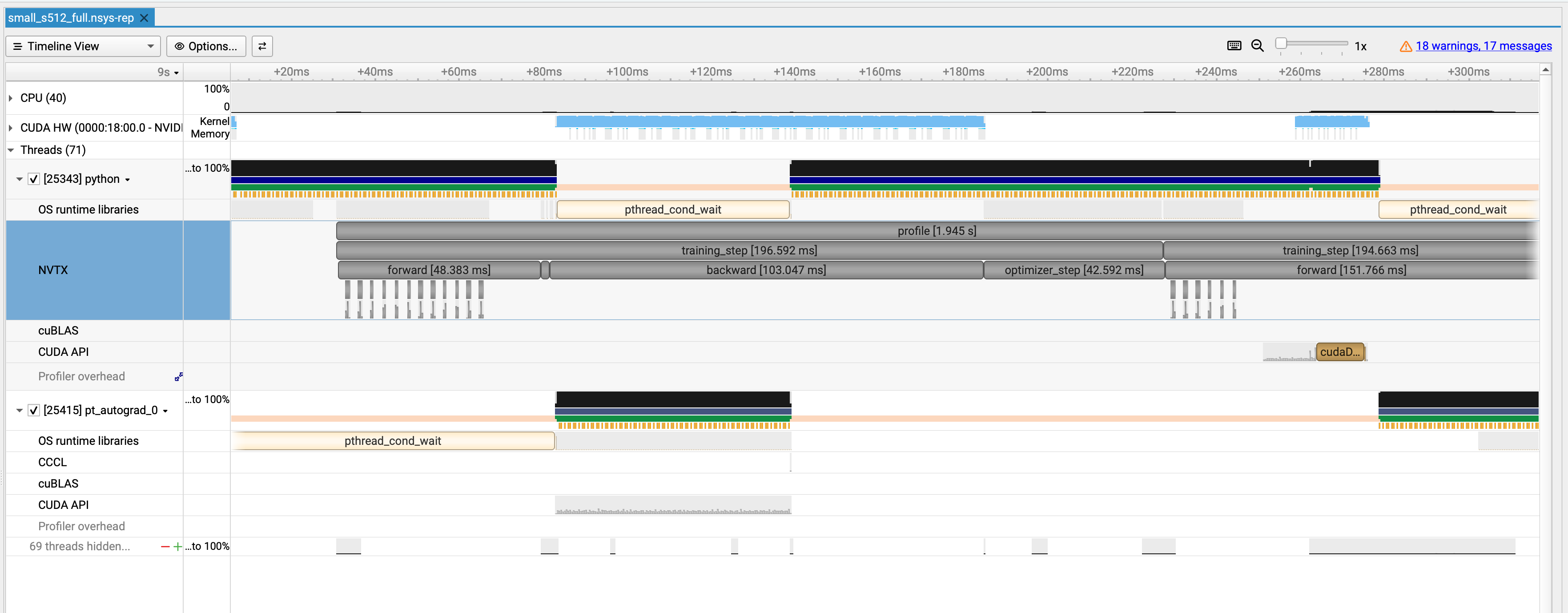
forward 中大致都是 48 ms（除了 step 2），和之前的同济保持一致

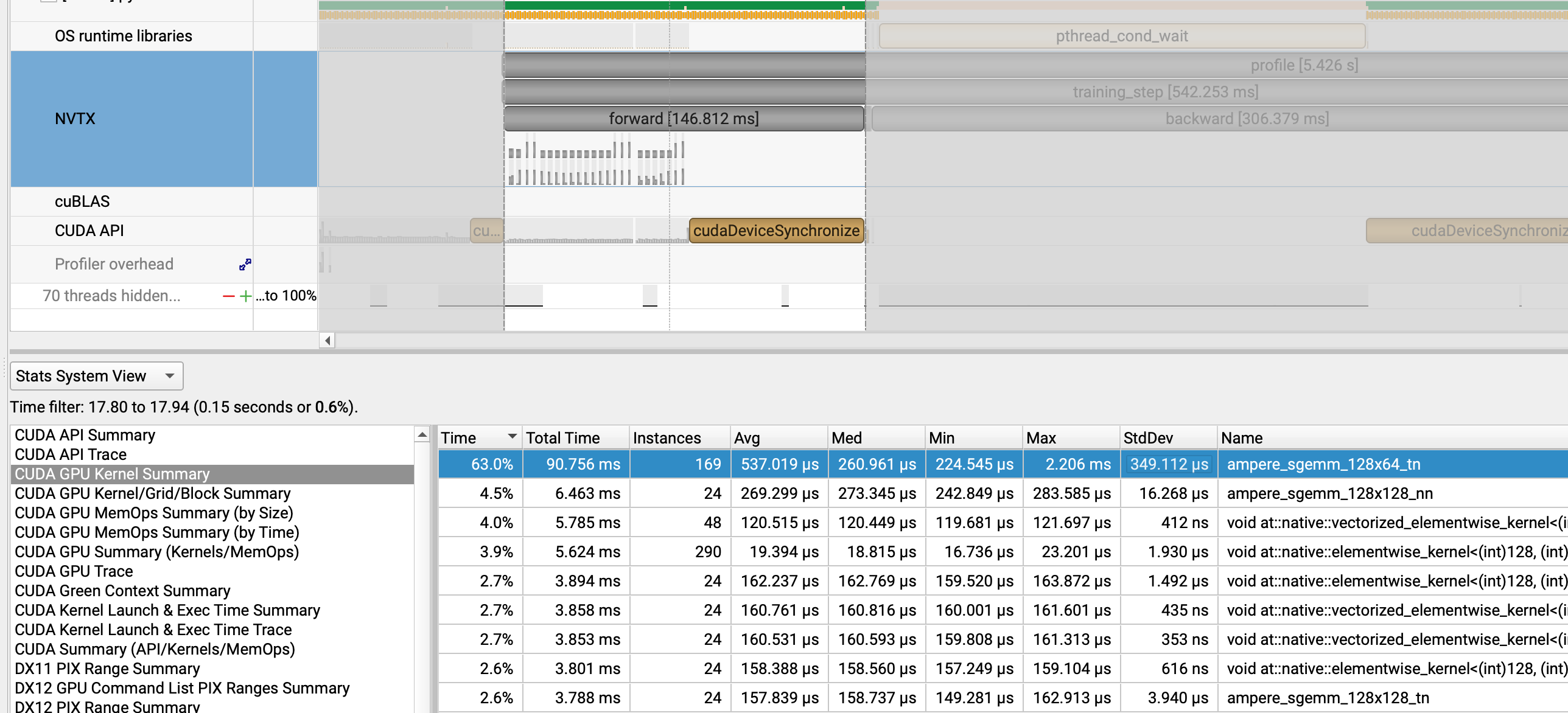
2. What CUDA kernel takes the most cumulative GPU time during the forward pass? How many times is this kernel invoked during a single forward pass of your model? Is it the same kernel that takes the most runtime when you do both forward and backward passes? (Hint: look at the “CUDA GPU Kernel Summary” under “Stats System View”, and filter using NVTX ranges to identify which parts of the model are responsible for which kernels.)

选择 forward 区间并添加 filter，ampere_sgemm_128x64_tn 内核占用时间最长，这是一个矩阵运算 kernel，ampere 是安培架构（因为 GPU 用的是 3090），sgemm 是 Single precision (FP32) General Matrix Multiplication，tn 表示矩阵转置。

如果把 forward 和 backward 全算进去，同样这个 kernel 占用时间最长。

3. Although the vast majority of FLOPs take place in matrix multiplications, you will notice that several other kernels still take a non-trivial amount of the overall runtime. What other kernels besides matrix multiplies do you see accounting for non-trivial CUDA runtime in the forward pass?

BinaryFunctor ... MulFunctor<float> 这一串就是非运算 kernel，用来向量访问内存。

4. Profile running one complete training step with your implementation of AdamW (i.e., the forward pass, computing the loss and running a backward pass, and finally an optimizer step, as you’d do during training). How does the fraction of time spent on matrix multiplication change, compared to doing inference (forward pass only)? How about other kernels?

在一个完整的训练步骤中 ampere_sgemm_128x64_tn 的占比是 9.1%，在 推理 forward 过程中占比为 32.6%。

5. Compare the runtime of the softmax operation versus the matrix multiplication operations within the self-attention layer of your model during a forward pass. How does the difference in runtimes compare to the difference in FLOPs?

softmax 耗时 161 微秒，attention score 计算耗时 175 微秒。

Attention 计算 $QK^T:(N\times d)(d\times N)$ 为 $2N^2d$ FLOPs，对 $N \times N$ softmax大约可以算作为 $N^2$。

在如此量级差距下，运算时间几乎相近，可能是由于 GPU 对大规模矩阵乘法的优化。

Mixed Precision

1. Suppose we are training the model on a GPU and that the model parameters are originally in FP32. We’d like to use autocasting mixed precision with FP16. What are the data types of:（具体项目参见下方回答）

1. the model parameters within the autocast context? 全都是 torch.float32
2. the output of the first feed-forward layer (ToyModel.fc1)? torch.float16
3. the output of layer norm (ToyModel.ln)? torch.float16
4. the model’s predicted logits? torch.float16
5. the loss? torch.float16
6. the model’s gradients? 全都是 torch.float32

2. You should have seen that FP16 mixed precision autocasting treats the layer normalization layer differently than the feed-forward layers. What parts of layer normalization are sensitive to mixed precision? If we use BF16 instead of FP16, do we still need to treat layer normalization differently? Why or why not?

实际上 autocast 没有自动上升到 FP32。但是 LN 中确实有对精度较为敏感的区域。

LN 中计算 $\sigma^2=\frac1N\sum_i(x_i-\mu)^2$ 之后需要就算根号 $\hat x_i=\frac{x_i-\mu}{\sqrt{\sigma^2+\epsilon}}$ 这一步对精度要求高。

LN 还是建议使用 FP32，即便 BF16 解决了动态范文，但是在计算累加过程中以及求均值时候，仍然会因为精度产生较大的误差。

3. Modify your benchmarking script to optionally run the model using mixed precision with BF16. Time the forward and backward passes with and without mixed-precision for each language model size described in Section 2.1.2. Compare the results of using full precision versus mixed precision, and comment on any trends as model size changes. You may find the nullcontext no-op context manager to be useful.

fp32
 mode=full
forward: mean=577.90us, std=12.01us (50 steps)
backward: mean=1.24ms, std=32.97us (50 steps)
optimizer_step: mean=1.86ms, std=6.57us (50 steps)

autocast-fp16
 mode=full
forward: mean=492.77us, std=23.81us (50 steps)
backward: mean=1.90ms, std=40.07us (50 steps)
optimizer_step: mean=2.31ms, std=29.88us (50 steps)

autocast-bf16
 mode=full
forward: mean=497.18us, std=30.76us (50 steps)
backward: mean=1.76ms, std=43.16us (50 steps)
optimizer_step: mean=1.87ms, std=18.41us (50 steps)

用混合精度在 Forward 上会有稍微的优势。在计算量比较小的时候 AMP 的收益比较有限，可能受到固定转化等成本影响。

Profiling Memory

1. Add an option to your profiling script to run your model through the memory profiler.

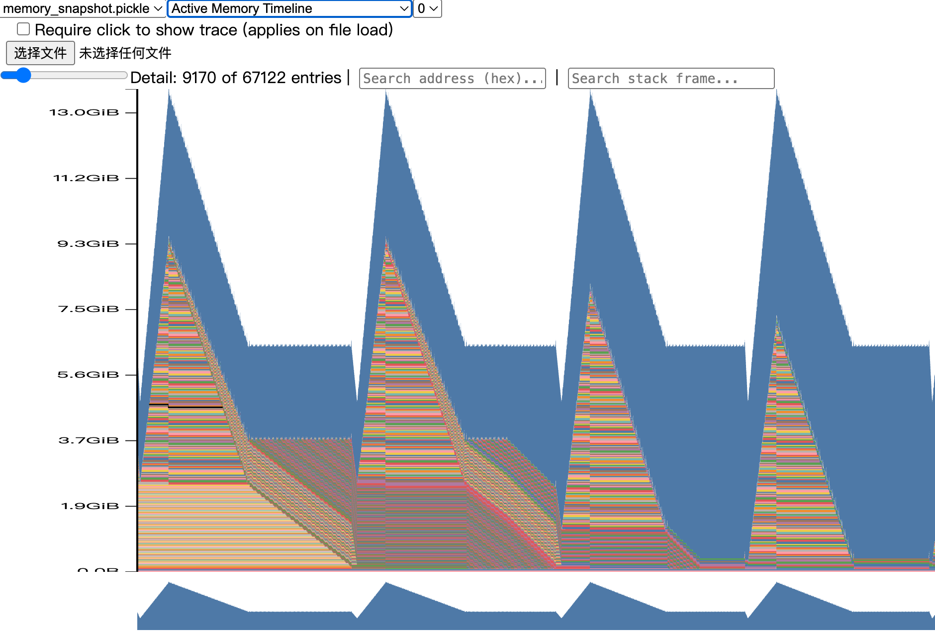
   It may be helpful to reuse some of your previous infrastructure (e.g., to activate mixed-precision, load specific model sizes, etc). Then, run your script to get a memory profile of the xl model when either doing inference only (just forward pass) or a full training step. What do your memory timelines look like? Can you tell which stage is running based on the peaks you see?

上图是训练全流程的大致图像长这样（显存不够，使用 medium 代替，后文同理），最大的峰值应该是 backward 开始了一段时间的时候，GPU 需要绝大多数的激活值来算 grad，还需要申请新 grad 的空间。

上图是仅 forward 的时候的显存占用，可以明显看到大量的内存从头到尾一直存在，没有被释放过，主要是模型本身的参数。

2. What is the peak memory usage of each context length when doing a forward pass? What about when doing a full training step?

见上文

3. Find the peak memory usage of the xl model when using mixed-precision, for both a forward pass and a full training step. Does mixed-precision significantly affect memory usage?

大致降低了显存的占用（train 阶段相比全精度，显存峰值减少了约 2 GiB），总体趋势没有改变。

4. Consider the xl model. Given our reference hyperparameters, what is the size of a tensor of activations in the Transformer residual stream, in single-precision? Give this size in MiB (i.e., divide the number of bytes by $1024^2$).

运行中 batch size 是 4，medium 中残差形状：$[B,T,d_{\text{model}}]$，计算为 $4\times512\times1024\times4 =8,388,608\text{ bytes} =8\text{ MiB}.$

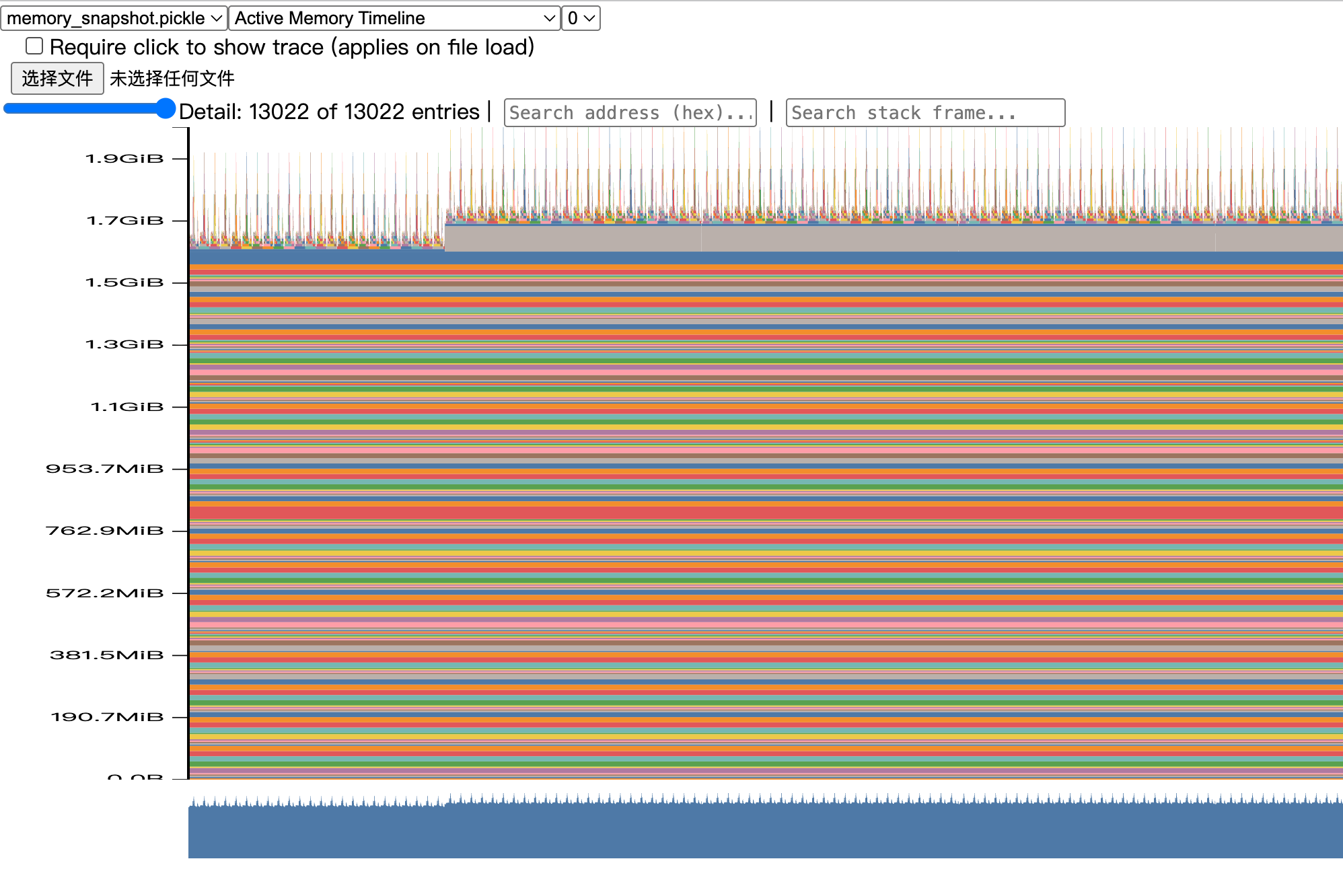
5. Now look closely at the “Active Memory Timeline” from pytorch.org/memory_viz of a memory snapshot of the xl model doing a forward pass. When you reduce the “Detail” level, the tool hides the smallest allocations to the corresponding level (e.g., putting “Detail” at 10% only shows the 10% largest allocations). What is the size of the largest allocations shown? Looking through the stack trace, can you tell where those allocations come from?

medium 中最大的内存块为 64MiB，锁定那一块内存，并阅读 trace（从下往上读）：

.../91_assignment_2/cs336-basics/cs336_basics/nn_utils.py:6:softmax
??:0:method_vectorcall.llvm.1911523193071396409
...91_assignment_2/cs336_systems/benchmark.py:41:annotated_scaled_dot_product_attention
??:0:method_vectorcall.llvm.1911523193071396409
...91_assignment_2/cs336-basics/cs336_basics/model.py:520:forward

可以看到是缩放点积中的 softmax 运算。考虑到Attention 计算中的 Attention score 矩阵大小为：$[B,H,T,T]$

$4\times16\times512\times512=16,777,216$ 个元素对应到 FP32 正好是 64 MiB

Single-GPU Memory

本节主要关注 Operation Fusion 的收益，减少为了 backward 而保留的中间值，也能加快运算速度。进一步，在 attention block 中的 attention map 有非常大的显存占用，所以引入了 Activation Checkpointing，也就是不再保留中间值，而是重新再算一遍 forward，是计算量与存储之间的 trade off。

checkpoint 越多，需要重计算的值越少，用于保存 input 的存储越多；checkpoint 越少，重计算的中间值越大，backward 的显存峰值会上升，但是保存的 input 会下降。两者之间会有一个中间点，使得显存值最小，构成最大化收益。以公式表达如下：

$$M(K) = O\left(\frac{N}{K}+K\right)$$

是一个经典的对钩函数。其中 $K$ 是 ckpt 数量，$O(K)$ 表示每一个 block 运算时候的 residual ，$O\left(\frac{N}{K}\right)$ 需要为 ckpt 保存的输入。

进一步，checkpoint 内部可以构成递归形式，让一个 checkpoint 本身不用保存全部的 residual，代价就是更多的 recompute，更多的内容会被重复计算。

Consider a Transformer with $N$ identical blocks stacked sequentially. Without any checkpointing, all $N$ blocks’ worth of residuals are kept alive simultaneously, giving $O(N)$ peak activation memory. We have a free hand to wrap any subset of the forward pass in checkpoint, including nesting checkpoint calls inside one another.

1. What checkpointing strategy minimizes peak activation memory, ignoring the compute cost? Describe how you would arrange the checkpoint calls (a code sketch is fine), and give the asymptotic peak activation memory and compute of your strategy as a function of $N$. Assume the residuals saved by a single block dominate any per-checkpoint bookkeeping.

从复杂度的角度来算，如果不考虑计算量，最节约的是多重递归直到最小的单位。例如将 N 个 block 设置一个 ckpt，然后该块中进一步设置两个 ckpt，一直递归下去。

空间复杂度： $S(N)=S(N/2)+O(1)$ 的递推式，总共有 $\log_2 N$ 个节点，求和就是 $O(\log N)$ 空间复杂度（峰值，因为算完即可释放）

时间复杂度是累加的，不同于空间复杂度只需要考虑峰值，而且每一个节点都需要其下的所有节点的计算量，所以总共 $\log_2 N$，每个 $O(N)$ 计算量，总共为 $O(N\log N)$

2. Consider the xl model config with batch size 4 and sequence length 2048 as above. If you only have the time/compute budget to run one step of recomputation (meaning you may not nest checkpoint calls), what is the best checkpointing strategy to reduce peak memory? Profile your run’s peak memory to validate your hypothesis. Compare the peak memory of the next smaller and larger checkpointing block sizes to be sure.

显存不足，改用 medium 模型（24 层）、batch size 4、序列长度 512 测量。将相邻 block 均匀分组，每组使用一次 checkpoint，不嵌套。下表为 10 次训练步测量的平均值；显存数值是相对步前已分配显存的峰值增量，包含梯度等分配。

每组 block 数	分组数 $K$	峰值显存增量	前向与反向耗时
不使用 checkpoint	—	9.05 GiB	457.69 ms
3	8	2.63 GiB	617.51 ms
2	12	2.33 GiB	614.67 ms
1	24	2.03 GiB	602.49 ms

在该配置的已测方案中，每层单独使用 checkpoint 的峰值显存增量最低。相邻的较大分组（每组 2 层）增加了 0.30 GiB

GPU Kernels

Optimizing Attention with FlashAttention-2

1. Benchmark your attention implementation at different scales. Write a script that will:

   • Fix the batch size to 8 and don’t use multihead attention (i.e. remove the head dimension).

   • Iterate through the cartesian product of [16, 32, 64, 128] for the head embedding dimension $d$ model, and [256, 1024, 4096, 8192, 16384] for the sequence length.

   • Create random inputs $Q, K, V$ for the appropriate size.

   • Time 100 forward passes through attention using the inputs.

   • Measure how much memory is in use before the backward pass starts, and time 100 backward passes.

   • Make sure to warm up, and to call torch.cuda.synchronize() after each forward/backward pass.

   Depending on your GPU, some of these configurations are expected to run out of memory. Report the timings (or out-of-memory errors) you get for these configurations. At what size do you get out-of-memory errors? Do the accounting for the memory usage of attention in one of the smallest configurations you find that runs out of memory (you can use the equations for memory usage of Transformers from Assignment 1). How does the memory saved for backward change with the sequence length? What would you do to eliminate this memory cost?

以下为 batch size 8、FP32 的现有运行记录。耗时是 10 次测量的均值；显存列为运行期间的峰值已分配显存，单位 MiB。

$d$	序列长度	前向 (ms)	反向 (ms)	峰值显存 (MiB)
16	256	4.92	4.23	246.86
16	1024	7.22	12.44	984.41
16	4096	39.19	88.99	4665.88
16	8192	124.10	279.29	12406.76
16	16384	显存不足	—	—
32	256	4.75	8.01	249.37
32	1024	6.67	11.90	991.42
32	4096	42.41	90.96	4690.89
32	8192	126.26	285.29	12444.27
32	16384	显存不足	—	—
64	256	3.74	8.23	254.42
64	1024	7.57	15.53	1005.47
64	4096	41.92	96.27	4740.94
64	8192	134.87	295.00	12519.33
64	16384	显存不足	—	—
128	256	3.05	8.61	264.60
128	1024	8.27	17.01	1033.66
128	4096	52.05	107.56	4841.13
128	8192	149.95	323.84	12669.56
128	16384	显存不足	—	—

最小的显存不足配置为 $d=16$、序列长度 16384。一个 $[8,16384,16384]$ 的 FP32 注意力矩阵占 $8\times16384^2\times4=8$ GiB；分数和 softmax 权重等中间结果会进一步占用显存。反向传播需保存的注意力权重随序列长度按 $O(T^2)$ 增长。可用分块计算并在反向时重算注意力权重，避免保存完整矩阵。

Benchmarking JIT-Compiled Attention

torch.compile

1. Extend your attention benchmarking script to include a compiled version of your PyTorch implementation of attention, and compare its performance to the uncompiled version with the same configuration as the pytorch_attention problem above.

2. Now, compile your entire Transformer model in your end-to-end benchmarking script. How does the performance of the forward pass change? What about the combined forward and backward passes and optimizer steps?

Flash Attention